Plus42 : An Enhanced HP-42S Calculator Simulator
Home > Plus42

What it is
Plus42 is an advanced scientific programmable calculator, based on Free42.
Free42, in turn, is a complete re-implementation of the HP-42S scientific programmable RPN calculator,
which was made from 1988 until 1995 by Hewlett-Packard. Free42 is a complete rewrite and contains
no HP code whatsoever.
Plus42 builds on Free42 and adds: A Larger Display, with 8 rows and 22 columns (131x64 pixels)
by default, which the user may resize at will; Algebraic Expressions modeled after those used
on the HP-27S and HP-17B/19B; attached Units and unit conversions modeled after those used
on the HP-48/49/50 series; Directories for more organized storage of programs and variables;
TVM and amortization tables;
and two-dimensional Plotting of functions, with ability to zoom and pan, and find integrals
and roots from points in the plot.
Plus42 is an Open Source project. The executables and source code are
released under the terms of the GNU
General Public License, version 2.
All third-party code used in Plus42 is either in the public domain, or
licensed under terms compatible with GPLv2, or used with the authors'
permission.
Project Status
The latest release is 1.3.15.
If you're interested in what's been going on with Plus42,
see the project history.
If you have questions or comments about Plus42, you may use the Free42 & Plus42 discussion group.
Alternatively, you can contact me, Thomas Okken, via email at thomas@thomasokken.com.
You can find answers to some frequently asked questions in the Plus42 FAQ.
Donations
The Android and iOS versions of Plus42 are paid apps,
but the Windows, MacOS, and Linux versions are free downloads. Any donations
will help keep Plus42 going.
You may donate any amount you wish, large or small.
Donations are processed by PayPal.
Page Contents
Downloads
Documentation
Frequently Asked Questions
Downloads
 |
Android
Get it at Google Play.
Requires Android 4.4 or later.
|
 |
iOS (iPhone, iPad, iPod touch)
Get it from the App Store.
Requires iOS 12.0 or later.
|
 |
Windows
Download: Plus42Windows.zip
(32-bit)
Requires Windows Vista or later.
If Plus42 does not run as is, you will also need to download and install the
Latest supported Visual C++ Redistributable.
For Windows versions before 10, you need older versions of the Visual C++ redistributable,
which you can find here.
|
 |
MacOS
Download: Plus42Mac.zip
Requires MacOS 10.13 (High Sierra) or later.
|
 |
Linux
Download: Plus42Linux.tgz
Built in Ubuntu 18.04, with libc 2.27, libstdc++ 8.4.0, and GTK+ 3.22.30.
It should work on any Linux (x86_64) with those or similar libraries.
|
Additional Downloads
|
 |
Skins
Some skins to use instead of the faceplates built into Plus42.
Note: Plus42 can use skins designed for Free42 as well. Find them here.
|
 |
HP-42S/Free42/Plus42 programs
A small collection of HP-42S/Free42/Plus42
programs. |
 |
raw2txt, txt2raw
Command-line tools that convert "raw" program files to text listings and back.
Downloads for Windows,
MacOS,
and Linux.
Last Updated: Apr 26 2025
|
 |
rom2raw
A C program that converts user code from HP-41 ROM images, from ROM or MOD files,
to Free42/Plus42/Emu42 compatible "raw" program files.
Download rom2raw.zip; source code
and Win32 console executable included.
|
 |
Plus42 Source Code
Get it from Codeberg: https://codeberg.org/thomasokken/plus42desktop
Package for GTK only, for building Linux packages: upstream.
I cannot keep track of exactly which combinations of tools do and don't work for building
Plus42, but for what it's worth, these are the ones I use:
- For the MacOS version, I always use the latest Xcode.
- For the Windows version, I use Microsoft Visual Studio 2026 with the VS 2022 SDK (v143).
- I have built the GTK version in many different Linux distros, and
also in FreeBSD and Solaris. What I typically need to install are: the
standard set of build tools (called 'build-essential' in Ubuntu),
libgtk-3-dev, libasound2-dev, and, if 'make' is not GNU Make, also
'gmake'. Note that libasound2-dev is optional; you just need it if you
want BEEP and TONE to sound nice.
|
Plus42 Documentation
Contents
Introduction
 Plus42 is a calculator app for people who like the simplicity and ease of use
of RPN keystroke-programmable calculators like the HP-42S, but also enjoy some
of the advanced features of HP's RPL series. It is an evolution of Free42,
which also continues to be maintained as a separate app. Plus42 is fully
compatible with Free42 and the HP-42S. Everything in the HP-42S and Free42
documentation fully applies to Plus42, so to get a complete picture of what
Plus42 can do, you should not just read this web page, but the Free42
documentation page as well.
Plus42 is a calculator app for people who like the simplicity and ease of use
of RPN keystroke-programmable calculators like the HP-42S, but also enjoy some
of the advanced features of HP's RPL series. It is an evolution of Free42,
which also continues to be maintained as a separate app. Plus42 is fully
compatible with Free42 and the HP-42S. Everything in the HP-42S and Free42
documentation fully applies to Plus42, so to get a complete picture of what
Plus42 can do, you should not just read this web page, but the Free42
documentation page as well.
Plus42 is not an attempt to re-create the RPL calculators in full. These machines
have a very well-thought-out design of their own, and if you want all their
functionality, before too long you are bound to find yourself replicating their
entire user experience. But it is possible to borrow some of their
functionality into an HP-42S-like calculator, without compromising the
elegance, simplicity, and intuitiveness of the 42S design.
I started adding some advanced functionality to Free42 in 2019: SST→ and SST↑
for easier debugging of large programs; LSTO for creating local variables;
a large RTN stack, which, in combination with LSTO, enables implementing
recursive functions; FUNC, RTNERR, RTNYES, and RTNNO, which make it possible
to write user-code functions which behave more like built-in ones; and finally,
a dynamically growing RPN stack.
These new functions are rather unobtrusive: if you don't need them and aren't
interested in them, you probably won't even notice they exist, and you can
continue using Free42 as an HP-42S-compatible calculator, just like before. And
if you do like them, you can use them to help with some of the more demanding
programming tasks, in a way that fits seamlessly with legacy code.
But there were also some ideas for improvements, floating around in the HP
calculator community, that would have much more of an impact on the user
interface, not to mention requiring much more work to implement. In 2021, with
time on my hands thanks to a certain global health crisis, I started work on
a fork of Free42, with the goal of adding support for algebraic equations,
attached units, directories, and a big display. And about a year later,
Plus42 1.0 was done.
If you are familiar with RPN programmable calculators, you will find Plus42
easy and intuitive to use. If you are familiar with the HP-42S specifically,
you'll be up and running almost immediately.
If you are not familiar with RPN calculators, I recommend starting by reading
the first few chapters of the HP-42S manual. Plus42 is an HP-42S simulator at
heart, and everything you read in that manual applies to Plus42 as well. And I
also recommend reading the documentation section of the Free42 home page (link); this covers loading and saving
programs, Copy and Paste, and loading and saving state files.
If you are interested in programming, you'll want to read the Extensions
section of the Free42 home page (link); this covers the advanced
programming features I mentioned above, and also some other functions not
present in the original HP-42S, like functions for accessing the current time
and date, and calculating with times and dates, and support for user-selectable
word sizes for the BASE menu functions.
What follows is documentation for the features present in Plus42 that are not
in Free42. Since much of this functionality is modeled after other HP
calculators, specifically, the HP-17B/19B/27S and the HP-48/49/50 series,
experience with those models will help, but it is not required.
Algebraic Equations
 In addition to keystroke programming like on the HP-42S and in Free42, Plus42 supports algebraic
equations. These can be used with the SOLVER, ∫ f(x), and PLOT application menus, and they can
be embedded in programs; they can be stored in variables and on the stack, and evaluated from
any of those contexts.
In addition to keystroke programming like on the HP-42S and in Free42, Plus42 supports algebraic
equations. These can be used with the SOLVER, ∫ f(x), and PLOT application menus, and they can
be embedded in programs; they can be stored in variables and on the stack, and evaluated from
any of those contexts.
The Plus42 equations, their syntax and capabilities, and the equation editor, are all
modeled after the Solver found on the HP-17B, 19B, and 27S calculators. The HP-17B
manual, sections 11 and 13; the HP-19BII manual, sections 11, 12, and 13; the HP-27S
manual, section 5; the HP-27S/19B Technical Applications book; and Martin Hepperle's
"About The Solver in the HP Pocket Calculators" — these can all be used with
the Plus42 solver, with only minor differences. The set of built-in functions provided
by Plus42 is a superset of the aforementioned calculators, and the direct and iterative
solvers are both implemented.
Note: The HP-17BII and HP-19BII manuals are available from the HP web site.
HP-17BII: http://h10032.www1.hp.com/ctg/Manual/c00442250.pdf
HP-19BII: http://h10032.www1.hp.com/ctg/Manual/c00442254.pdf
Equation Mode
The heart of the Plus42 equation functionality is Equation Mode, which is the
central place where you enter and edit equations, and perform calculations with
them.
You enter Equation Mode by pressing the EQN key on the keyboard, or using the
= key in the SOLVER, ∫ f(x), and PGMMENU menus.
This takes you to the Equation List.
In the Equation List, the two rightmost menu buttons are ↑ and ↓ buttons. These are used to
rearrange equations: they swap the current equation with the one just above or
below in the list. If the display is set to show just two rows, ↑ and ↓ will briefly show the
equation being swapped with, and then move to the new position in the list, so
you are left looking at the same equation as before.
If you want to move through the list without rearranging it, use the familiar ▲
and ▼ buttons.
To add a new equation, you can press NEW and start typing, or Paste text from a
different app. The new equation or equations will be inserted after the current
one.
If you pressed NEW, you will see the familiar ALPHA menu for entering text. To
move the cursor to a different position, press EXIT to go to the cursor
movement menu; this has keys for cursor movement in all four directions, plus
DEL to delete the character under the cursor (to delete the character to the
left of the cursor, press the backspace key on the keyboard), and ALPHA to go
back to the ALPHA menu. Pressing EXIT from the cursor movement menu will finish
editing and return you to the Equation List.
To start editing an existing equation, select it using ▲ and ▼ and press EDIT.
This puts you in the Equation Editor, just like NEW, except you start in the
cursor movement menu, rather than the ALPHA menu.
Use DELET to delete the current equation. Use this with caution: once an
equation has been deleted, it cannot be recovered!
When you press DELET, and some or all of the variables used by the equation
exist, you will be offered the choice whether to delete just those variables,
or just the equation, or both.
Last but not least, press CALC to start performing calculations with the
currently selected equation.
The action of CALC depends on how you entered Equation Mode. If you used EQN,
or = in the SOLVER menu, CALC performs EQNSLV and
enters the SOLVER menu; and if you used = in the
∫ f(x) menu, CALC performs EQNINT and enters the ∫ f(x) menu. Once
in these menus, you use them with the current equation, exactly like you would
if you had selected a program.
You can change the action of CALC without leaving Equation Mode, by pressing
Shift-7 or Shift-8 (SOLVER and ∫ f(x)). You will briefly see a message
confirming the new action.
Summary of List View
This is the complete list of all the keys that are active while in the list view:
CALC and ENTER Start calculating with
the currently selected equation.
EDIT Start editing the currently selected equation. The
equation editor is discussed in detail below.
DELET Delete the currently selected equation. Since this
is a rather drastic operation, you will be asked for confirmation; also, if any
of the variables used by the equations exist, you will be asked whether you want
to delete those variables only, the equation and its variables, or the equation
only. Deleting the variables only can be a convenient way of resetting your
calculations.
NEW Start editing a new equation. The equation will be
inserted in the list below the currently selected one.
↑ and ↓ Move the currently selected
equation up or down in the list, swapping it with the equation just above or below.
Shift PLOT Exit equation mode and
enter the PLOT menu, with the current equation selected as if using EQNPLOT.
STO Export the equation to the RPN calculator environment.
You will be offered these options: X to push the equation onto the stack,
placing it in the X register; PRGM insert it into the current program as
an XSTR line; if the current program line is an XSTR line, you will be offered the
choice of overwriting that line, or inserting a new XSTR after it; if the current
program line is not an XSTR, the equation is always inserted after it; and
ALPHA, which puts the equation in the ALPHA register. When storing in ALPHA,
bear in mind that the ALPHA register can only hold up to 44 characters, and equations
can be any length, so any given equation may not fit.
RCL Import an equation from the RPN calculator environment.
You will be offered these options: X to get it from the X register;
PRGM to get it from the current program line; and ALPHA to get it
from the ALPHA register.
Shift MODES and
Shift DISP The normal MODES and
DISP menus; the settings in these menus affect the equation environment much like
the RPN environment, so access to them is provided here, without having to leave
equation mode.
▲ and ▼ Move the selection up or
down one position in the list view. When pressed with Shift,
jump directly to the beginning or end of the equation list.
Shift SOLVER Set SOLVE mode, so
pressing CALC or ENTER will enter the SOLVER menu with the currently selected equation.
Shift ∫ f(x) Set INTEG mode, so
pressing CALC or ENTER will enter the ∫ f(x) menu with the currently selected equation.
Shift PRINT Opens the PRINT menu.
This menu is a bit different than the PRINT menu shown in the RPN environment. This
menu is discussed separately, below.
EXIT Exit equation mode and return to the RPN environment.
Shift OFF Exit the Plus42 app.
The Equation Mode PRINT Menu
The PRINT menu in Equation Mode is accessible both in the List View and in the Equation
Editor. It has different functions than the PRINT menu in the RPN environment:
EQ Prints the current equation.
LISTE Print the whole equation list.
VARS Prints the variables used by the current equation.
LISTV Print all variables.
PRST Print the RPN stack.
ADV Paper advance; prints a blank line.
The second row of the PRINT menu has the printer mode settings: PRON, PROFF, MAN,
NORM, TRACE, and STRACE; these work the same as the third row of the RPN-mode
PRINT menu.
The Equation Editor
When you press EDIT or NEW in the equation list view, you enter the Equation Editor.
This is a very basic text editor. It is similar to ALPHA mode, except in the equation
editor, there is no 44-character length limit, and you can move the cursor around freely.
The two main menus in the equation editor are the cursor movement menu and the ALPHA
menu. When you press EDIT, you will start with the cursor movement menu, and when you
press NEW, you will start with the ALPHA menu, but you can switch between these two
menus at any time: from the ALPHA menu, pressing EXIT will take you to the cursor movement
menu, and from the cursor movement menu, pressing ALPHA will take you to the ALPHA menu.
The cursor movement menu exists in two variations, and which one you see depends on
the current display size. The standard case is when the display has three or more
rows, in which case the menu will look like
DEL
←
↑
↓
→
ALPHA
and when the display has two rows, it will look like
DEL
<←
←
→
→>
ALPHA
In two-line mode, there are no "up" and "down" arrows, since there is only one line
of text being displayed; in other words, the view is like the equation is all on
one line, no matter how long it may be. The <← and →> menu keys move left
and right by one screenful at a time. And in both two-line and multi-line modes,
pressing Shift with a cursor movement key moves as far as
you can go in the given direction: to the top or bottom of the text, or to the left
or right margin, or to the beginning or the end.
Because of their importance in equations, the characters ( ) [ ] . , = : are
assigned to keys of their own in the equation editor, so you don't have to go through
the ALPHA menu to type them.
The parentheses, ( and ), are used to control precedence, and to
delimit lists of parameters passed to functions; [ and ] are used
for indexing matrices and lists; . and , are used as the decimal,
interchangeably and independent of RDX. / RDX, mode (note that
thousands separators are not allowed in equations); =, when used
at the top level of an equation, asserts the equality between the left-hand
and right-hand sides of an equation, and in conditional contexts, is the equality
test operator; and : is used as a separator, separating the elements in
parameter lists, separating the indexes in two-dimensional matrix indexing, and
separating the elements in Σ(), ∫ (), IF(), FOR(), and SEQ() expressions and
matrix literals.
While in the equation editor, these menus are available: UNITS, the stack menu (R↓),
MATRIX, STAT, BASE, CONVERT, hyperbolics (FLAGS), PROB, CUSTOM, PGM.FCN, PRINT,
TVM, and CATALOG. The PRINT menu was discussed in the sub-section above; all the
other menus only serve the purpose of allowing you to enter functions into
equations without having to spell them out letter by letter. Most of these menus
have slightly different contents than their RPN-mode counterparts, showing only
those functions that can be used in equations, and, in some cases, functions that
are available only in equations.
Equation Syntax and Semantics
The syntax and semantics is closely modeled after the HP-17B and its siblings.
In particular, all the functions listed in Martin Hepperle's "About The Solver
in the HP Pocket Calculators" have been implemented.
These characters are special in the equation language:
+ - × ÷ ^ ↑ ( ) < > = : * / [ ] { } ! _
That means they cannot be used as part of identifiers (i.e., variable or function
names). In addition, the digits 0 through 9, and the characters
. , ᴇ, that is, the number characters, can be used in identifiers, but
not as the first character of identifiers.
In compatibility mode, the characters * / [ ] { } ! _ lose their special
meanings, and can be used in identifier names. This mode is intended for
compatibility with the HP-17B, 19B, and 27S calculators, where these characters
have no special meaning and are commonly used in variable names. There are
straightforward alternatives for most uses of these characters: instead of
*, you can use ×; instead
of /, you can use ÷; instead of A[B], you can use
ITEM(A:B); instead of A != B, you can use A <> B;
instead of A_"B", you can use UNIT(A:"B"); and instead of
{A:B:C}, you can use APPEND(NEWLIST:A:B:C).
On the other hand, the lack of [ ] means you cannot enter matrix
literals, and will have to create empty matrices using NEWMAT, and then use code to populate them.
The equation language defines the following operators, shown in decreasing order
of precedence:
| ( ) [ ] { } | Grouping; parameter passing; matrix and list indexing and literals |
| ^ ↑ _ | Exponentiation and unit attachment |
| × * ÷ / | Multiplication and division |
| + - | Addition and subtraction; unary plus and minus |
| = ≠ <> != < ≤ <= > ≥ >= | Comparisons |
| NOT | Logical NOT |
| AND | Logical AND |
| OR XOR | Logical OR and XOR |
| = | Equality assertion (top level only) |
Expressions operate on variables, number literals, string literals, and matrix literals.
- Variables have names of 1 to 7 characters in length, subject to the character
restrictions mentioned above. Note that the 7-character maximum is less than the 10-character
maximum on the HP-17B and other HP calculators; this is because in Plus42, variables in equations
correspond to named variables in the RPN environment.
- Number literals consist of one or more decimal digits, with an optional decimal period or comma,
and an optional exponent. The exponent must be introduced with one of e E ᴇ and consists
of one or more decimal digits, optionally preceded by a + or - sign. Note that
strictly speaking, there are no negative number literals; a number like -2 is actually
a 2 with a unary minus applied.
- String literals consist of a sequence of zero or more characters, enclosed in "
signs. Within a string, the escape sequences \" and \\ are used to denote "
and \.
- Matrix literals have the form [[A11:A12:A13]:[A21:A22:A23]:[A31:A32:A33]].
Elements can be any expression that evaluates to a real number or string. Row vectors are written as [[A:B:C]]
and column vectors as [A:B:C], the latter being a shorthand for [[A]:[B]:[C]].
- List literals have the form {A:B:C}.
Elements can be any expression, including matrices or other lists.
Equations may optionally be named, by prefixing them with a name followed by a colon, or a name
followed by an argument list, then a colon. For example: PYTHAGORAS:A^2+B^2=C^2 or
ACCELERATED_MOTION(T):X0+V0*T+A*T^2/2.
These names can be used simply to identify equations to the user, but they can also be used
to refer to equations from other equations, that is, named equations can be called by other
equations, similarly to calling functions.
Equation names are not subject to the 7-character name length restriction for variable names.
Since equation variables correspond to Plus42 named variables, they can have any of the
types that Plus42 variables can, including real numbers without units, real numbers with units,
complex numbers, real and complex matrices, strings, and lists.
Matrices and lists can be indexed using square bracket notation or using the special ITEM() function.
For matrices, one- or two-dimensional indexing can be used; for lists, only one-dimensional indexing
is used. When a matrix is indexed using a single index, the matrix elements are numbered left-to-right
and top-to-bottom.
Indexes start from 1, in both one- and two-dimensional indexing. And when lists are indexed for
writing, they are resized as needed, so that the assignment succeeds. So, for example, when
L(M[10]:5) is executed and M is a list, if it has fewer than 10 elements,
it will be resized to 10, so the assignment can succeed. This automatic resizing is not
performed while reading from a list, and it is never performed for matrices.
Compatibility Mode
There are a few differences between the equation language of Plus42 and the equation language of
the HP-17B and other HP calculators. For compatibility with the HP calculators, Plus42 has
a compatibility mode, which can be turned on using the COMP setting in the MODES menu. The standard
Plus42 mode is STD.
These differences exist between standard and compatibility modes:
- In compatibility mode, the characters * / [ ] { } ! _ may be used in variable names;
in standard mode, * is an alternate spelling of the multiplication operator ×,
/ is an alternate spelling of the division operator ÷, [ ] are
used for matrix literals, and for indexing, with A[B] being an alternate syntax for
ITEM(A:B), ! is used to write !=, which is an alternate spelling of
<> or ≠, _ is used to attach units to numbers, with A_"B"
being an alternate syntax for UNIT(A:"B"), and { } are used for list literals.
- In compatibility mode, L() and G() cannot see local variables, like the loop variable
defined by the first parameter of Σ(). In standard mode, L() and G() can see all variables.
Whether an equation is parsed in standard or compatibility mode can be selected globally
using the STD and COMP settings in the MODES menu. When an equation is parsed in STD mode,
the resulting equation object is shown with straight single quotes as delimiters, while
when an equation is parsed in COMP mode, the resulting equation object is shown with
backquotes as delimiters. Note that STD/COMP mode only takes effect during parsing; the
parsed equation object will keep its behavior even if the STD/COMP mode setting is changed
after the equation was parsed.
It may be desirable to mark certain equations for STD or COMP parsing regardless of the
global STD/COMP mode setting, for example, if you have mosly STD-type equations where you
make full use of Plus42 syntax, but also need to use a small number of COMP-type equations
that were originally written for HP calculators, and would be inconvenient to adapt to
Plus42 syntax.
To force an equation to be parsed in STD mode, regardless of the global STD/COMP mode setting,
simply add :STD: between the function name and the function itself, or add :COMP:
for functions that should always be parsed in COMP mode. For functions without names, add the
:STD: or :COMP: at the beginning, for example: :STD:function or name:STD:function
or name(x:y:z):STD:function, and similarly for :COMP:.
Functions
The equation language provides the following built-in functions:
SIN(X) COS(X) TAN(X)
ASIN(X) ACOS(X) ATAN(X) | Trigonometric functions and their inverses |
SINH(X) COSH(X) TANH(X)
ASINH(X) ACOSH(X) ATANH(X) | Hyperbolic functions and their inverses |
| DEG(X) RAD(X) | Radians-to-degrees and degrees-to-radians conversions
(RPN: →DEG →RAD) |
LN(X) LNP1(X) LOG(X)
EXP(X) EXPM1(X) ALOG(X) | Natural logarithm, natural logarithm of X+1,
and base-10 logarithm, and their inverses
(RPN: LN LN1+X LOG E↑X E↑X-1 10↑X) |
| SQRT(X) SQ(X) | Square root; square
(RPN: SQRT X↑2) |
| INV(X) | Reciprocal
(RPN: 1/X) |
| FACT(X) GAMMA(X) | Factorial and Gamma functions
(RPN: N! GAMMA) |
| COMB(X:Y) PERM(X:Y) | Number of combinations or permutations of Y elements from a set of X |
| PI π | The mathematical constant π |
| RAN# | Returns uniformly distributed pseudo-random numbers greater than 0 and less than 1
(RPN: RAN) |
| ABS(X) | Absolute value |
| SGN(X) | Sign function: for real numbers, returns +1 for positive numbers,
0 for zero, −1 for negative numbers, and z/|z| for complex numbers. Note that this
is different from the RPN function SIGN in that the latter returns 1 for zero. |
| INT(X) IP(X) FP(X) | Round to integer toward negative infinity; round to integer
toward zero; return fractional part of X, equivalent to X−IP(X) |
| IDIV(X:Y) MOD(X:Y) | Integer division and remainder |
| RND(X:Y) TRN(X:Y) | Round-to-nearest, or round-to-zero, the number X, to Y decimal
digits (if Y nonnegative) or to −Y significant digits (if Y negative) |
| DATE(X:Y) | Calculate the date Y days after date X
(RPN: DATE+) |
| DDAYS(X:Y:C) | Calculate the number of days between dates X and Y, using calendar
C, where 1 = Gregorian Calendar, 2 = Calendar without leap days, and 3 = 30-day calendar
(RPN: C=1 corresponds to the RPN function DDAYS) |
| CDATE CTIME | Returns the current date; current time
(RPN: DATE TIME) |
| HMS(X) HRS(X) | Convert decimal hours to hours, minutes, seconds, and the reverse
(RPN: →HMS →HR) |
| HMSADD(X:Y) HMSSUB(X:Y) | Add or subtract times or angles in hours, minutes, and
seconds
(RPN: HMS+ HMS−) |
SIZEC(X) SIZES(X)
MROWS(X) MCOLS(X) | Returns the size of a cash flow list; size
of a regular list or the number of elements of a matrix; number of rows of a matrix;
number of columns of a matrix |
| DEC(X) OCT(X) | Octal-to-decimal and decimal-to-octal conversions
(RPN: →DEC →OCT) |
BNOT(X) BAND(X:Y)
BOR(X:Y) BXOR(X:Y) | Bitwise logical operations NOT, AND, OR, XOR
(RPN: NOT AND OR XOR) |
BNEG(X) BADD(X:Y) BSUB(X:Y)
BMUL(X:Y) BDIV(X:Y) | Binary arithmetic operations
(RPN: BASE+/− BASE+ BASE− BASE× BASE÷) |
| INVRT(X) DET(X) | Returns the inverse or determinant of the square matrix X |
| TRANS(X) | Returns the transpose of the matrix or vector X |
| DOT(X:Y) CROSS(X:Y) | Dot and cross product |
| FNRM(X) | Returns the Frobenius norm of the matrix or vector X |
| RNRM(X) | Returns the Row norm, or the row sum norm, of the matrix X (this is
the maximum of the 1-norms of its rows) |
| RSUM(X) | Returns the vector of sums of each of the rows of the matrix X |
| UVEC(X) | Returns the unit vector for the complex number X, or if X is a vector
or matrix, returns X/FNRM(X) |
| NEWLIST NEWMAT(R:C) | Create a new list, or a new matrix with R rows and C columns.
Note that NEWLIST does not take any arguments; it always returns an empty list. Lists are
resized as needed, whenever they are written to. |
NN→S(X) N→S(X) S→N(X) N→C(X) C→N(X)
APPEND(X:Y:...) EXTEND(X:Y)
HEAD(X) TAIL(X)
LENGTH(X)
POS(X:Y) POS(X:Y:Z) SUBSTR(X:Y)
SUBSTR(X:Y:Z) REV(X) | List and
string functions. These simply correspond to the RPN functions with the same names, except for
APPEND, HEAD, and TAIL.
APPEND can take 2 or more parameters, with the first being a list
and the remaining parameters being any type, and adds the second and subsequent parameters to
the end of the list, each parameter being added as a separate element.
HEAD(X) returns the
first element of the list or string X, or {} or "" if the list or string
is empty.
TAIL(X) returns the list or string X, with its first element or character
removed, or {} or "" if the list or string is empty. |
| #T(X:Y) FLOW(X:Y) | Return the Yth count or the Yth flow from cash flow list X |
| ITEM(X:Y) ITEM(X:Y:Z) | Return the Yth element from list or matrix X, or the
element at row Y and column Z from the matrix X. Equivalent to X[Y] and X[Y:Z], but works
even in compatibility mode. |
| RCOMPLX(RE:IM) PCOMPLX(R:PHI) | Construct a complex number using real part RE
and imaginary part IM, or using magnitude R and angle PHI. Note that internally, complex
numbers are always represented in rectangular form. |
RADIUS(RE:IM) RADIUS(Z)
ANGLE(RE:IM) ANGLE(Z) | Get the magnitude and angle
of a complex number, which may be provided either as separate real and imaginary parts,
or as a complex number object. |
XCOORD(R:PHI) XCOORD(Z)
YCOORD(R:PHI) YCOORD(Z) | Get the real and imaginary
parts of a complex number, which may be provided either as a separate magnitude and angle,
or as a complex number object. |
| UNIT(X:Y) | Construct a unit object from a real number X and a unit string Y.
equivalent to X_Y, but works even in compatibility mode. |
| UBASE(X) | Converts X to its base unit. |
| UVAL(X) | Returns the value of X, discarding its unit, if any. |
ΣX ΣX2 ΣY ΣY2 ΣXY ΣN
ΣLNX ΣLNX2 ΣLNY ΣLNY2
ΣLNXLNY ΣXLNY ΣYLNX | Statistics sums,
accumumated by the RPN Σ+ function (read-only) |
| MEANX MEANY SDEVX SDEVY WMEAN | Mean of X and Y; sample standard
deviation of X and Y; weighted mean of X with weights Y; for the data accumumated by
the RPN Σ+ function (read-only) |
| CORR SLOPE YINT FCSTX(X) FCSTY(X) | Correlation coefficient, slope, Y intercept,
and backward and forward forecasting, using the statistics sums the RPN Σ+ function
and the currently selected fitting model. CORR, SLOPE, and YINT are read-only; FCSTX and
FCSTY behave like normal invertible functions.
| N(I%YR:PV:PMT:FV:P#YR:BEGIN)
I%YR(N:PV:PMT:FV:P#YR:BEGIN)
PV(N:I%YR:PMT:FV:P#YR:BEGIN)
PMT(N:I%YR:PV:FV:P#YR:BEGIN)
FV(N:I%YR:PV:PMT:P#YR:BEGIN) | TVM:
Calculate N, I%YR, PV, PMT, or FV, in terms of the other four, with P#YR the number of payments per
year, and BEGIN=1 for payments at the beginning of the period, and BEGIN=0 for payments at the end. |
SPPV(I:N) SPFV(I:N)
USPV(I:N) USFV(I:N) | Present and future value of a unit,
with interest rate I and N periods, for Single Payment or Uniform Series. |
| REGX REGY REGZ REGT LASTX STACK[N] | Read-only access to the RPN stack |
| MIN(X1:X2:...) MAX(X1:X2:...) | Return the smallest or largest of its
arguments. Any number of arguments is allowed. |
| REAL?(X) CPX?(X) MAT?(X) CPXMAT?(X) STR?(X) LIST?(X) EQN?(X) UNIT?(X) TYPE?(X) | Test
whether X is a real number, a complex number, a matrix (real or complex), a complex matrix,
a string, a list, an equation, or a number with an attached unit; return an integer indicating
the type of X, like the RPN TYPE? function |
| Σ(VAR:FROM:TO:STEP:EXPR) | With the variable VAR going from FROM to TO in steps of STEP,
calculate the sum of evaluating EXPR once for each value of VAR. |
| ∫(EXPR:VAR:LLIM:ULIM:ACC) | Integrates the expression EXPR with integration variable
VAR going from LLIM to ULIM, with relative accuracy ACC. The ACC parameter is optional; if
omitted, the value of the variable ACC will be used, if it exists, or otherwise, the integral
will be calculated with maximum precision. |
| IF(A:B:C) | If A is 'true', returns B, else C. |
FOR(INIT:COND:NEXT:EXPR:...)
BREAK CONTINUE | After evaluating the initialization
expression INIT, starts executing these steps in a loop: first, evaluate COND, and if it
returns 'false', exit the loop; evaluate EXPR and any additional expressions that follow;
evaluate NEXT; repeat. When it finishes, FOR returns the value returned by the last EXPR to be
evaluated, or the value returned by INIT if the loop body was never executed at all, that is,
if COND returned 'false' the first time it was called.
Within the list of expressions EXPR:..., the special expressions BREAK and CONTINUE
may be used. BREAK ends the FOR loop immediately, and CONTINUE ends the current execution of
the EXPR:... list, proceeding to NEXT and the next iteration. |
| SEQ(EXPR1:EXPR2:...) | Evaluates EXPR1, EXPR2, etc., in sequence, and returns the
value that was returned by the last expression. This may be used when multiple expressions
need to be evaluated in a context that normally allows only one. |
| XEQ(NAME:X1:X2:...) | Calls the user code program starting with LBL "NAME". The
parameters X1, X2, etc., will be assigned to the MVAR parameters declared by the program, or
pushed onto the stack if the program has no MVAR declarations. The return value will be
whatever is left in the X register when the program returns. |
| EVALN(NAME:X1:X2:...) | Calls the equation stored in the variable named "NAME". The
parameters X1, X2, etc., will be assigned to the equation's declared parameters. |
| FunctionName(X1:X2:...) | Calls the equation named FunctionName
in the equation editor's list. The parameters X1, X2, etc., will be assigned to the
equation's declared parameters. |
| STOP(X) | Inserts a STOP in the generated code. Meant for debugging.
In terms of function evaluation, it simply returns its argument unchanged, and it is
invertible. |
| VIEW(EXPR1:EXPR2:...) | Inserts VIEW instructions in the generated code, one for
each argument. Meant for debugging. Use with PRON mode if you want the values of EXPR1 etc.
to be sent to the printer, or use with PROFF mode and flag 21 set if you want the execution
to halt on each VIEW, to be resumed manually using R/S.
In terms of function evaluation, it behaves like SEQ(). |
L(NAME:VALUE)
G(NAME) | Assign the value VALUE to the variable named NAME, or
get the value of the variable named NAME. In STD mode, this works on all variables,
including the local variables created by Σ() and when calling named equations; in COMP
mode, L() and G() only work on global variables.
NAME may be an array element, so you can say things like L(A[B]:C). Note that when
writing to a list in this way, the list will be expanded, as needed, to make sure index
B exists.
| | LL(NAME:VALUE:EXPR:...) | Create a local variable with name NAME and initialize it
with the value VALUE, and then execute the expressions while the local variable is in scope.
The return value of LL() is the value returned by the final expression.
| | S(NAME) | Returns 'true' if SOLVE is currently active, and NAME is
the variable currently being solved for; returns 'false' in all other situations. |
|
Notes About Parsing in EQN Mode
You may have noticed that equations
are stored in the EQNS list in parsed form, but how and when do functions actually get parsed?
The answer is that equations are always parsed before being stored in EQNS, and,
if necessary, they are parsed again by CALC.
Equations can be stored in EQNS in three ways: by exiting the equation editor
without cancelling; by pasting into the equation list; and by inserting an
equation into the equation list using RCL. In each of those cases, Plus42 will
attempt to parse the equation, and if successful, it will store the resulting
equation object in EQNS. If the parse is not successful, it will not report
an error, but instead simply store the equation as an unparsed string, so you
can revisit and correct it later.
When CALC is pressed, and the currently selected equation is an unparsed
string, it will then attempt to parse the string, and if successful, store
it in EQNS; if the parse fails, an error will be reported, since CALC absolutely
needs a parsed equation in order to proceed.
If the currently selected equation is a parsed equation object,
it is used as is. However, there is one additional case, where the equation
will be parsed again, even though it had already been parsed successfully,
and that is the case where the global compatibility mode setting has changed
(STD or COMP in the MODES menu; see the section about Compatibility Mode, above).
This behavior ensures that equations without embedded :STD: or :COMP: tags will
always behave in accordance with the current STD or COMP mode setting when
used by CALC, while also making sure that equations aren't parsed any more
often than necessary. This last consideration is significant because
equation objects include not just the equation text, but also associated
data structures and generated code. This means they are rather heavyweight
data structures, and they should be reused and shared whenever possible.
When equation objects are copied (using ENTER, DUP, STO, RCL, etc.), the copies
actually all point to the same internal data structures, so once an equation
object is created by PARSE, creating additional copies of it is a very
inexpensive operation. But if an equation string is parsed again and again,
each parse operation creates a brand new equation object, and there is no
sharing in that case. Thus, it makes sense to parse an equation as soon as
possible and then copy the parsed equation object as necessary, and the
behavior of EQN with regards to parsing is designed with this in mind.
Direct vs. Iterative Solver
When SOLVE is used with equations, it will try to apply the direct solver first.
The direct solver works by rearranging the equation, so that the variable to
be solved for is isolated by itself on one side of the equals sign.
This works by using substitutions like these (assuming the variable to be solved for is X):
    F(X)=Y → X=Finv(Y)
    F(X)+Y=Z → F(X)=Z-Y
    Y^F(X)=Z → F(X)=LN(Z)/LN(Y)
    etc.
This approach only works if the variable to be solved for occurs only once in
the equation, and if all the functions that have to be inverted have explicit
inverses, and if no divisions by zero occur during the rearrangement.
If the direct solver can't be used, SOLVE will fall back on using the numeric
solver instead. This is the same solver that is used for solving programs.
The HP-27S and HP-17B/19B manuals refer to it as the iterative solver.
You may force SOLVE to always use the numeric solver, by setting NUMERIC mode
in the MODES menu. To allow the direct solver to be used, set DIRECT mode
instead. (DIRECT mode is the mode that is initially set, when the calculator is first
turned on.)
Equation Execution and Debugging
 When an equation is parsed, whether automatically in EQN mode or explicitly using
the PARSE function, Plus42 generates a program. When the equation is evaluated,
it is this program that is actually executed.
When an equation is parsed, whether automatically in EQN mode or explicitly using
the PARSE function, Plus42 generates a program. When the equation is evaluated,
it is this program that is actually executed.
Normally, you do not have to be aware of the generated code. However, when
errors occur during the execution of an equation, it can be useful to understand
what is happening behind the scenes.
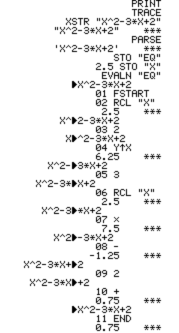
You can see the generated code in action if you evaluate an equation with TRACE
mode enabled. TRACE mode is a printer mode that causes every program step to
be printed, and its results. (See the HP-42S Owner's Manual, chapter 7, for
details.) When Plus42 executes an equation, TRACE mode prints not just the
program steps, but it also shows which part of the equation the current program
step corresponds to.
If you want to use SST to execute an equation step by step, you can use the
STOP() function to insert a breakpoint. The STOP() function becomes a STOP
instruction in the generated code. Once execution is stopped, you can use
SST to continue executing step by step, or R/S to continue running the
equation.
Alternatively, if you place an EVAL or EVALN instruction in a program, you
can SST into that instruction, and that way, you can SST the entire equation
from the start, without needing a breakpoint, just like when you SST an XEQ
in a program.
When an error occurs while evaluating an equation, the equation text surrounding
the location of the error is shown in the display. To see the location of the
error within the full equation, enter EQN mode and press R/S. This will locate
the equation where the most recent error occurred, load it into the equation
editor, and place the cursor at the site of the error.
Equations in Programs
Starting with Plus42 1.2.4, equations can be embedded in programs. There are two
types of equation program lines: plain lines and EVAL lines. A plain equation line
puts the equation object on the stack without evaluating it, while an EVAL
equation line evaluates the equation, without placing it on the stack.
    01 LBL "EQLINES"
    02 'A+B'       ; plain equation line, STD mode
    03 EVAL 'A+B'  ; EVAL equation line, STD mode
    04 `A+B`       ; plain equation line, COMP mode
    05 EVAL `A+B`  ; EVAL equation line, COMP mode
    06 END
(EVAL equation lines are functionally equivalent to equation lines in the HP-35s;
see the HP-35s manual, page 13-7.)
There are two ways to enter equation lines into a program: using STO in EQN mode,
and using X2LINE in PRGM mode.
When using STO in EQN mode, a check is performed whether the current program
line is an equation line or an XSTR, and if it is, you will be asked whether
you want to overwrite this line with the new equation line, or insert the
equation line after the current line. If the current line is not an equation
or XSTR line, the new equation line will always be inserted after it.
Next, you will be asked whether to insert a plain equation line or an EVAL line.
After you make your selection, the new equation line will be created.
The other way to create an equation line is to go into PRGM mode and use the
X2LINE function. The X2LINE function takes the contents of the X register and
inserts them into the program after the current line. This works for real numbers,
complex numbers, strings, and equations. When X contains an equation, a plain
equation line is created.
Note that X2LINE does not provide an option to create an EVAL line directly.
However, you can change plain equation lines into EVAL equation lines, or
vice versa, by executing EVAL while on the equation line.
Note that this makes it a bit more difficult to enter a plain equation line,
immediately followed by EVAL, into a program, since the EVAL function will change
the current equation line, rather than insert a normal EVAL instruction into
the program. You can work around this by first entering a dummy line after
the equation, then enter the EVAL, and finally, delete the dummy line.
Editing Equations on the Stack and in Programs
It is possible to create and edit equation objects without going through EQN mode.
For this purpose, there are these two functions in the EQN.FCN menu:
NEWEQN Starts the equation editor with an empty buffer.
When you leave the editor, you can save the equation as a string or as an
equation object. If you called NEWEQN in normal mode, the object will be pushed
onto the stack, and if you called NEWEQN in PRGM mode, the object will be inserted
into the program.
EDITEQN Starts the equation editor, loading the object
from the X register or the current program line into the buffer, depending on
whether you execute the function in normal mode or PRGM mode. When you leave the
editor, you can save the equation as a string or as an equation object, replacing
the original object.
Some Final Notes About Equations
Equations can be named with parameter lists: FUN(X:Y):X^2−2*X*Y+Y^2. Such
equations can be called like functions from other equations.
Functions may return complex results, depending on the HP-42S REALRES/CPXRES mode setting.
Equations can be shared with the RPN (HP-42S-based) environment using STO and
RCL in the list view. STO will offer to write the current equation to the X
register, ALPHA register, or current program location, and RCL can retrieve
equations from those same places.
In the RPN environment, equations may be used in much the same way programs
can, using a parallel set of functions: EVALN instead of XEQ, EQNSLV and EQNINT
instead of PGMSLV and PGMINT, EQNMENU and EQNMNU1 instead of VARMENU and
VARMNU1, and EQNVAR instead of PGMVAR.
You can also play with equations without ever using the equation editor: first,
create the equation as a string using XSTR, or by pasting the text from a text
editor; then use PARSE to convert the string in the X register to an equation
object. EVAL evaluates the equation object in the X register, and is exactly
equivalent to EVALN ST X.
Note that XSTR will only let you enter up to 50 characters when you use it
interactively, but when created by pasting text, XSTR commands in programs can
be up to 65535 characters long, and string objects (on the stack and in
variables) don't have a length limit at all.
Units and Conversions
 Plus42 supports numbers with attached units. For exampe, the quantity of two
and a half kilometers can be represented as 2.5_km, with number and unit
joined together. When calculations are performed with such number-unit pairs,
the necessary conversions take place automatically, and if an operation is
impossible because the units are incompatible — such as when trying to
add a length to an area — an error message is shown.
Plus42 supports numbers with attached units. For exampe, the quantity of two
and a half kilometers can be represented as 2.5_km, with number and unit
joined together. When calculations are performed with such number-unit pairs,
the necessary conversions take place automatically, and if an operation is
impossible because the units are incompatible — such as when trying to
add a length to an area — an error message is shown.
The Units Catalog
You can access units by pressing the UNITS key, or by selecting the UNITS
catalog in the CATALOG menu. The two are equivalent; the UNITS key is just a
shortcut to access the units catalog with fewer keystrokes.
The units catalog is divided into 16 sections, each containing units of similar
quantities: LENG for units of length, POWR for units of power, ELEC for various
electrical units, and so on.
You use the units in the units catalog by applying them to the number in the X
register. The X register must contain either a simple real number without a
unit, or a number that already has a unit; you cannot attach units to complex
numbers, matrices, or other types. To apply a unit to the number in the X
register, simply press its key. For example, if you're in the LENG section and
the X register contains the number 2.78, pressing cm applies the
centimeter unit, and the result is 2.78_cm.
You can combine units; for example, to enter "five Newton-meters", type
5 FORCE N EXIT LENG
m, to get 5_N*m. To divide by a unit instead of
multiplying, press Shift: to enter "55 volts per meter", type 55
ELEC V
EXIT LENG Shift m, to get 55_V/m. And
you can enter powers of units by entering them multiple times: to enter
"9.80655 meters per second squared", type 9.80655 LENG m EXIT
TIME Shift s Shift s, to
get 9.80655_m/s^2.
The real power of attached units lies in the fact that you can perform calculations
with them. The result of the calculation will have the appropriate unit, and any
necessary conversions will be performed automatically. For example, 25_m
3_s ÷ gives 8.3333_m/s.
When adding or subtracting, the result of the operation will have the same unit
as the number provided in the X register. So, for example, the result unit of
adding one foot and one meter depends on the order of the operands: 1_m
1_ft + gives 4.2808_ft, while 1_ft
1_m + gives 1.3048_m.
This behavior can be used to convert numbers to different units, by adding
zero with the desired unit attached. For example, to convert 12 miles to kilometers:
12_mi 0_km +, to get 19.3121_km.
When units are combined in multiplication or division, the resulting unit is
simplified by combining or cancelling identical units, but no conversions are
performed. This means that m^2 divided by m gives m, but
yd divided by ft gives yd/ft: while yards and feet are
compatible units, they are not identical, so they are not cancelled against
each other automatically. Of course, if you happen to know the
unit of the result, you can use conversion to force the unit to be normalized;
for example, if you already know that yd/ft is dimensionless, you can
simply add zero: 1_yd/ft 0 + gives 3,
or 1_acre*ft 0_gal + gives 325852.7320_gal.
Other ways of normalizing units are discussed below.
The UNIT.FCN menu contains a few functions that can be useful when working
with units, particularly when using units in programs, but also when using
units in manual calculations:
CONVERT Converts the number in the Y register to the
unit in the X register. Only the unit part of the number in the X register is
used; the value part is ignored.
In practice, it will usually be more convenient to add zero with the desired
unit, rather than use the CONVERT function.
UBASE Converts the number in the X register to its
base unit. All units defined in Plus42 are defined in terms of these base
units: m, s, kg, mol, K, A, r,
sr, and cd, and every derived unit can be expressed as some
unique combination of these base units. UBASE finds this unit and converts
the number in X to it.
UVAL Returns the value part of the number in X,
discarding its unit. No conversions are performed.
UFACT Factors out the unit in X from the number in Y.
Only the unit part of the number in the X register is used; the value part is
ignored.
Use this function if you want a unit to be expressed in terms of a specific
other unit. For example, say you have a speed in mph, and you want to
see it in terms of meters: 15_mph 0_m UFACT, to get 11.176_m/s.
→UNIT Applies the unit in X to the dimensionless
number in Y. Only the unit part of the number in the X register is used; the value part is
ignored. For example: 3.16 125_m →UNIT, gives 3.16_m.
UNIT→ Splits the number in X into its value (the same
value that is returned by UVAL) and its unit, attached to 1. For example,
40076_km UNIT→, gives 40076 in Y and 1_km in X. It is
valid to apply this to a number without a unit, in which case 1 will
be returned in X.
UNIT? Tests whether the object in the X register is
a number with a unit or not. This is a do-if-true conditional, meaning it
displays Yes or No, as appropriate, when executed from the keyboard,
or it either does not, or does, skip the next instruction, while running a program.
Spelling Out Units
Instead of using the UNITS catalog, you can also enter units by typing them
directly, letter by letter. This is only possible during number entry, and is
convenient primarily when using Plus42 on computers with a full keyboard.
To attach a unit to a number being entered, press Shift
.. An underscore will be appended to the number, which
may be hard to spot at first because the number entry cursor is also an
underscore. Once you do this, the ALPHA menu will be activated, and you can
then enter the unit letter by letter. Bear in mind that units are case-sensitive,
so don't type KM when you mean km.
If you want to cancel entering the unit, you can backspace until you're back
at the number part, or press EXIT to remove the unit all in one go. When finished
entering the unit, press ENTER; this only ends number entry, but does not perform
the usual RPN duplication of the X register.
User-Defined Units
You can define your own units, and use them just like the pre-defined ones.
These user-defined units can be derived units, that is, defined in terms of
pre-defined units and/or other user-defined units; or they can be base units,
not defined in terms of anything else, and not touched by UBASE.
To define a derived unit, simply create a number that represents the value
of 1 of that unit, and then store it as a variable, giving it the name
you want to use for the unit.
For example, to define "pond", a customary Dutch unit equal to half a kilogram,
do 0.5_kg STO "pond". To see that this works, try converting 15 pond
to kilograms: 15_pond 0_kg +, to get 7.5_kg.
You may define dimensionless constants by using the unit one, which
simply represents the number 1. For example, to define tau, a
constant sometimes used to represent 2π, do 2_one π
× STO "tau".
For easier entry, you can assign user-defined units to the CUSTOM menu. This
works like any other assignment: ASSIGN "pond" TO 01, ASSIGN "tau" TO 02, etc.
When a unit is assigned to CUSTOM, you can multiply by that unit by simply
pressing its key, or divide by that unit by pressing Shift
followed by its key. And you can convert to that unit as you would with any
other unit, by attaching it to 0 and then adding.
To define a base unit, store the special value 0_one. User-defined
base units behave just like pre-defined base units. For example, let's define
a base unit named USD, to represent U.S. Dollars: 0_one STO "USD", and then
calculate the cost of 10 yards of fabric, sold at a price of 5 dollars per
foot: 5_USD/ft 10_yd ×, gives 50_USD*yd/ft;
normalize: UBASE, gives 150_USD.
Note that since user-defined units are simply variables, a user-defined unit
only works as long as it is visible. This means you'll probably want to store
your user-defined units in the HOME directory, or in a directory that is included
in the PATH list. See the section on directories for more information about
directories and variable lookups.
Assigning units to the CUSTOM menu
It is possible to assign units to the CUSTOM menu. Once assigned, they work just
like the units in the UNITS menu: when you press a menu key with a unit assignment,
the unit is applied to the value in the X register, and when you press Shift and
then the menu key, the unit is removed from the value in the X register (or
rather, the value in the X register is multiplied or divided by the unit,
respectively).
In the previous section, it was explained how this works when assigning user-defined
units. Those assignments are really a special case of variable assignments, but
it is also possible to assign built-in units, or compound units made up of
combinations of built-in and/or user-defined units. For example, ASSIGN "km" TO 01
assigns the built-in km unit to the first CUSTOM menu item, and this
assignment will work without a variable named "km" having to exist.
Unit assignments are looked for after all the other types of assignments. The
complete sequence of events inside the calculator when a CUSTOM menu key is
pressed is as follows: 1. Look for a LBL, and if found, XEQ it. 2. Look for
a variable; if found and it is a unit, apply it, and if it is any other type
of variable, RCL it. 3. Look for a built-in function, and if found, perform
it. 4. Check if the assignment matches a built-in unit, or if it is a
compound unit made out of built-in units and/or existing user-defined units, and
if so, apply it. 5. If none of the previous 4 steps were successful, XEQ
the assignment as if it were a LBL; since the LBL doesn't actually exist,
the end result will be a Label Not Found error message.
Final Notes on Units
Units work with arithmetic (including STO and RCL arithmetic), 1/X, X^2, SQRT,
and Y^X (integer and 1/integer exponents only), %, %CH, IP, FP, RND, ABS, SIGN,
MOD, SOLVE, INTEG, and PLOT. They cannot be stored in matrices or numbered
registers, but they can be stored in named variables and lists.
With Y^X with 1/integer exponents and SQRT, all the units must have powers
divisible by the exponent, since units with non-integral exponents are not
allowed, unlike on HP calculators. Also, SIN, COS, TAN, →REC, and COMPLEX in
POLAR mode will recognize angles with angular units and treat them
appropriately, ignoring the current angle mode.
Units are supported in equations. The syntax is slightly different from units
in normal RUN and PRGM modes, in that the units must be enclosed in double
quotes. So, instead of 16_oz, you write 16_"oz". What's going on
here is that the units are actually string literals, and _ is a
multiplicative operator that creates a unit object from a number on its left
and a string on its right.
In compatibility mode, _ is an identifier character, so it's not
available to use as an operator; in this case, the syntax UNIT(16:"oz")
can be used instead.
Directories
 In Plus42, internal storage is organized in directories. A directory can contain programs,
variables, and other directories. There is always at least one directory, called HOME, which
is created when the app creates a new state, and which cannot be deleted.
In Plus42, internal storage is organized in directories. A directory can contain programs,
variables, and other directories. There is always at least one directory, called HOME, which
is created when the app creates a new state, and which cannot be deleted.
Because of the importance of directories, the path of the currently active
directory is always displayed at the top of the screen. Initially, it will say { HOME },
but when you create and change directories, it will show a list of directories, always
starting with HOME and ending with the name of the current directory, with the chain of
ancestor directories in between.
Use DIRS to navigate the directory hierarchy. DIRS actually opens
a special section of CATALOG, which you can also reach using the CATALOG menu. The DIRS
catalog provides a view of the current directory; it allows you to move between
directories, in addition to showing you the programs and variables that are in the current
directory.
Unless you're looking at the HOME directory, the DIRS catalog always starts with
.., which moves to the parent directory
of the current directory; the HOME directory is at the top of the directory hierarchy, so
it has no parent.
Following the .., also shown on black keys, are the current directory's
sub-directories, if there are any. Next, shown on white keys, are the programs in the current
directory; this is the same list that you see when you press GTO. And last, shown on black
keys, are the variables that exist in the current directory; this is the same list that you
see when you press RCL.
When you press a directory key, the selected directory becomes the current directory; when
you press a program key, an XEQ to the corresponding LBL or END is performed; and when you
press a variable key, that variable is RCLed. And when you press Shift
followed by a directory, program, or variable key, a Reference to that item is created
and placed on the stack; references and their uses are discussed later in this section.
Directories are manipulated using commands found in the DIR.FCN menu. It contains these
functions:
CRDIR (or MKDIR) Creates a new directory. This directory will become a child
of the current directory.
CHDIR Changes into a subdirectory. The selected directory will
become the new current directory. This is also the action that is performed when you press
a directory key in the DIRS catalog.
UPDIR Changes into the current directory's parent directory. This
is also the action that is performed when you press the .. key in
the DIRS catalog.
HOME Changes into the HOME directory. Remember, HOME is the un-deletable
and un-renamable top of the directory hierarchy.
PATH Returns the path to the current directory, as a string
formatted like HOME:FOO:BAR:BAZ, in which BAZ is the current directory, BAR is
the current directory's parent, FOO is BAR's parent, and so on until HOME.
RENAME Renames a directory. To rename the directory FOO, located
in the current directory, to BAR, place the string "BAR" in the ALPHA register, and then
perform RENAME "FOO". Note that moving a directory to a different directory requires a
different function; this is discussed later in this section.
PGDIR (or RMDIR) Deletes ("purges") a directory. This will delete the named
directory and all its contents, including sub-directories, so use this with caution!
PRALL Prints a summary of all directories and their contents,
in a hierarchical, indented format. Programs are shown with their sizes, and variables
are shown with their types, and, in the case of matrices and lists, also their sizes, but
the contents of programs and variables are not shown.
All operations that access programs or variables operate primarily within the current
directory, but programs and variables in ancestor directories will also be found, for
operations that don't modify or delete their targets. So, for example, if no variable
named "A" exists in the current directory, RCL "A" will look for it in the ancestor
directories as well, and similarly, XEQ "Q" will look for LBL "Q" in ancestor directories
if it isn't found in the current directory. But STO "A" will always create or update the
variable "A" in the current directory; even if "A" does not exist in the current directory
but does exist in an ancestor directory, STO "A" will create a new variable "A" in the
current directory, leaving the "A" in the ancestor directory alone.
Operations that read and modify their targets will only work when their targets
are in the current directory. So, for example, attempting to edit a program
that isn't in the current directory will result in a Restricted Operation
message, and attempting to modify a variable that isn't in the current
directory will result in a Variable Not Writable message. Specifically,
Variable Not Writable will happen with STO+, STO−, STO×, STO÷, X<>, ISG,
DSE, and HEAD.
Directory, program, and variable management
Sometimes, you may want to move items from one directory to another, or create copies.
Plus42 supports these kinds of operations using Reference objects.
In the DIRS catalog, pressing Shift followed by a directory item
generates a "reference" object. This is a type of object that contains no data of its own,
but only acts as a pointer to something else. This is similar to a "shortcut" or
"symbolic link" in desktop environments.
Creating a reference object while there is already a reference in the X register
causes a list object to be created, with both reference objects inside. Creating further
reference objects adds them to this list, while creating a reference that is already on
the list removes it from the list. This functionality exists to make it convenient
to create sets of references, which you can then move or copy all at once.
Note that you can even add references to objects from multiple directories to the same
list, so this is a very flexible and powerful means of creating selections.
These reference objects, and lists containing only reference objects, serve one and only
one purpose: they can be fed to the new REFMOVE, REFCOPY, and REFFIND functions.
(Actually, that is not quite true; directory references are also used in the PATH
list. This is covered later in this section.)
REFMOVE Moves the referenced objects into the current
directory. In case of a list, the objects are added in the order in which they
appear in the list, and they are added in front of the already existing
objects. Note that it is possible to move objects within a directory as well,
which can be useful if you want to change the order in which they appear in the
catalogs.
REFCOPY Works like REFMOVE, except it copies items
instead of moving them. However, directories and variables within the current
directory are never copied, always just moved. (Programs are copied.)
REFFIND Finds the real object referenced by the
reference in X. (This only works when X contains a single reference object, not
a list.) It changes to the referenced directory, and moves to the referenced
program or VIEWs the referenced variable.
For convenience, the REFMOVE, REFCOPY, and REFFIND commands are mapped to the
keyboard when objects of the appropriate types are in the X register; REFMOVE
is −, REFCOPY is ×, and REFFIND is
÷.
For example, let's say you have variables A, B, and C, which you want to move
from directory FOO to directory BAR, and both FOO and BAR are children of HOME.
Here is how you could accomplish this: DIRS, then press
.. until you're at HOME, then press FOO
to go to the FOO directory; Shift A
Shift B Shift
C (there will now be a 3-item
list in the X register); .. BAR
(to go to the BAR directory); − (REFMOVE, to move the
three items to BAR).
A few more words about the reference objects themselves:
References are created by pressing Shift followed by a
DIRS menu item. Pressing a directory item causes a directory reference to be
created, and pressing a LBL or END item causes a program reference to be
created, and pressing a variable item causes a variable reference to be
created. Pressing Shift .. is special: it causes a reference
to the current directory to be created, not to the parent directory as you might
expect.
Reference objects can only be used as input for REFMOVE, REFCOPY, and REFFIND,
as mentioned above, but the way they are displayed is designed to at least make
it reasonably obvious to the user just what they are referring to. This works
as follows:
Directory references look like Dir[2] "HOME". The word Dir indicates
the type of reference, and the number in square brackets is the directory ID. This
ID is assigned to a directory when it is created, and it never changes, even if the
directory is moved or renamed. The name that is shown after the Dir[ID]
part is the current name of the directory with that ID; the name is not actually a
part of the reference object. So, if you create a directory reference, and then
rename that directory, the reference object will be displayed with the updated name.
The point is that the name is only shown for the convenience of the user.
(Note: directory ID 2 is the HOME directory. All other directories will have
numbers greater than 2. The number 1 is used internally to represent an invisible
directory, where generated code for equations is stored; and numbers ≤ 0 are
used internally to represent levels on the RTN stack where local variables are
stored.)
Program references look like Pgm[5:1] "FOO". The word Pgm
indicates the type of reference; the first number in square brackets is the ID of
the directory where the program is located, and the second number in square
brackets is the index of the program within that directory. The name that is
shown after the Pgm[ID:Index] part is the first global label found in
that program; for programs that don't contain any global labels, END
or .END. is shown instead.
As with the directory names shown in directory references, the global label names
shown in program references are only shown for the convenience of the user. They
aren't actually part of the reference objects themselves. Also, note that
when you insert or delete programs, references to programs with higher indexes
within that same directory will end up pointing at other programs. Unlike
directory IDs, which never change, program indexes simply represent the positions
of programs in their containing directories, and those positions can change.
Variable references look like Var[5:"A"]. The word Var indicates the
type of reference; the number is the ID of the directory of the variable is
located, and the name is simply the variable's name. Unlike with directory and
program references, where the directory or label names aren't actually part of
the reference objects and only shown for the convenience of the user, the names
in variable references are part of the reference; these names are how
they are represented to the user and how the system keeps track of them
internally. This is the reason why the variable names are shown inside the
brackets, to highlight the fact that they are a part of the reference objects
themselves.
The PATH Variable
(Not to be confused with the PATH function!)
As was mentioned earlier, operations that perform read-only access to programs
and variables, like GTO and RCL, will look for their targets in the current directory
first, but if they don't find them there, will also try the current directory's ancestors,
up to and including HOME.
For programs and variables that you want to be able to access from anywhere, you can
use the PATH variable. This is a list, which the system looks for in the HOME directory,
containing references to directories. If a program or variable was not found in the
current directory or its ancestors, the directories in PATH are tried next, from first
to last. (If PATH contains items that aren't directory references, they are simply
ignored.)
(Note: Actually, the above isn't the whole story. When a running program performs a
GTO or XEQ to a global label, and it isn't found during the search of the current directory
and its ancestors, the next step is to look for it in the directory where the currently
running program resides, and its ancestors. Only when that second search has
also failed to find the label, will the PATH list be searched.
Note that this only applies to label searches, and only from running programs.)
Directory Searches vs. Command Completion Menus
Many functions, including GTO and RCL but also most other functions that access global
labels or named variables, will pop up a menu of eligible labels or variables for the
user to choose from, so they don't have to be spelled out each time. In Plus42, these
menus will show eligible items from the current directory on black menu buttons, and
any eligible items from ancestor directories, or from directories referenced by the
PATH list, using white menu buttons. Note that the list of eligible items will depend
on the operation being performed, so RCL may show items from ancestor directories, but
STO or CLV never will.
Current Program vs. Current Directory
The current program is the program you'll see when you enter PRGM mode, and that will
execute when you press R/S or SST. The current directory is where functions like GTO
and RCL will start looking for global labels and named variables.
What can be confusing is that the current program isn't necessarily in the current
directory. When you change directories using CHDIR, the current program does not
change along with it, and conversely, when the current program is changed by GTO or
XEQ, the current directory does not change along with it, either.
You can tell when the current program is not in the current directory when you switch
to PRGM mode. If the triangle that indicates the current program line is solid black,
the current program is in the current directory; if it is a hollow triangle,
the current program is not in the current directory. The distinction matters,
because you can only edit programs that are in the current directory.
If you are looking at a program and are unable to edit it because it isn't in the
current directory, performing GTO .
. will change the current directory to the program's directory.
You can see the effect because the hollow triangle will turn solid black, and the
directory shown in the header will change. Or, approaching it from the other side,
when you perform GTO "label" while not in PRGM mode, the current directory will automatically
be set to the directory where the target LBL was found.
Note: It is possible to step into generated code, that is, programs that are created by
Plus42 when it parses equations. For example, if you execute a program fragment like
XSTR "A+B*C" PARSE EVAL, the PARSE will translate the equation to an RPN program, and
store it in the invisible directory with ID 1, and EVAL will call that generated code,
somethat like XEQ. When you SST the EVAL, you will next find yourself single-stepping
the generated code.
This is perfectly legal and safe, but you will not be able to use the
GTO . .
trick to make directory 1 the current directory, and start editing the
generated code. When in generated code, GTO .. simply does what it usually
does, which is to create a new empty program at the end of the current
directory, and make that the current program.
Big Display
 When Plus42 creates a new state, by default it now creates a display with 8 rows by 22 columns.
The DISP menu contains several functions for adjusting and querying the display size. They are:
ROW+ and ROW− Increase or
decrease the number of rows. The minimum number of rows is 2 and the maximum is
99.
COL+ and COL− Increase or
decrease the number of columns. The minimum number of columns is 22 and the
maximum is 999.
GETDS and SETDS Get or set
the display size. GETDS returns the number of rows in Y and the number of
columns in X, and SETDS sets the display size. The number of rows passed to
SETDS must be between 2 and 99, and the number of columns must be between 22
and 999. Unlike ROW+, ROW−, COL+, and COL−, GETDS and SETDS are programmable.
WIDTH and HEIGHT Get the
display size, in pixels. The main use of these functions is to make programs
that use PIXEL and AGRAPH resolution-independent: instead of hard-coding the
display width as 131 and the display height as 16, as you would when
programming Free42 or the real HP-42S, use WIDTH and HEIGHT, and you can make
your programs work regardless of the screen size that happens to be in effect.
This kind of modification works perfectly with the DPLOT program from the
HP-42S Owner's Manual, for example.
HEADER This function turns the information header on
or off. The header shows the current directory, and also the BEGIN/END and P/YR
mode, while the TVM menu is active, and the word size and signed/wrapped modes,
while the BASE menu is active. It is only shown when the number of rows is set
to 4 or greater, but it can be disabled altogether using this function, to free
up even more room for stack or program display.
1LINE and NLINE These
functions control how matrices and lists are displayed, when they are in the
X register and the number of display rows is set to 3 or greater.
In 1LINE mode, matrices and lists are shown in compact format, that is,
like [ 25x1 Matrix ] or { 3-Elem List },
which is the format used in Plus42 before release 1.0.17.
In NLINE mode, they are shown expanded, so you can actually see their contents
without needing to print them or having to use EDIT.
Note that objects in the other stack registers / levels are always displayed
in compact format, and everything is shown in compact format when the
display is set to 2 rows.
LTOP Toggle display of LASTX at the top of the stack area.
ATOP Toggle display of ALPHA at the top of the stack area.
HFLAGS Toggle display of flags 0-10 in the header.
HPOLAR Toggle display of POLAR mode in the header.
STK Toggle between full-screen matrix / list editing and normal stack display.
Financial Functions
 Plus42 has a TVM menu, containing functions for Time Value of Money calculations,
and to calculate and print amortization schedules. This functionality is closely
modeled after the TVM menu found on the HP-17B, but should also be familiar to
anyone who has used the HP-19B or its variants.
Plus42 has a TVM menu, containing functions for Time Value of Money calculations,
and to calculate and print amortization schedules. This functionality is closely
modeled after the TVM menu found on the HP-17B, but should also be familiar to
anyone who has used the HP-19B or its variants.
N, I%YR, PV,
PMT, and FV The standard functions
for compound interest. Entering a number and pressing one of these keys stores the
number, while pressing one of these keys right after another one calculates the
quantity from the other four.
A simple example: If you borrow $10,000 at 5% annual interest, and make monthly
repayments of $100, how long will it take to pay off the loan?
Shift DISP FIX 02
Shift TVM
5 I%YR 10000 PV −100 PMT
(note: PV is positive because it is money you receive, and PMT is negative because it is
money you pay; you could change the sign of both numbers, performing the calculation from
the point of view of the lender)
0 FV N
Result: 129.63, or 130 monthly payments, that is, 10 years and 10 months.
CLEAR Clears N, I%YR, PV, PMT, and FV, setting them all to zero.
P/YR Sets the number of payments per year.
BEGIN and END Select whether payments
are made at the beginning or at the end of each period.
RESET Sets P/YR to 12 and selects END mode.
AMORT Enters the amortization menu.
With the amortization menu, you can calculate and print amortization schedules,
where you can see how much of your payments go toward interest and how much
toward the principal, and see the remaining balance. The calculations can be
performed in steps of one or more periods. The initial values for the calculation
are taken from the I%YR, PV, and PMT settings from the main TVM menu, taking the
same P/YR and BEGIN/END settings into account.
For example, to calculate an amortization schedule for the same $10,000 loan used in
the example above:
AMORT
Result:
#P=1 PMTS: 0-0
Interest=0.00
Principal=0.00
Balance=10,000.00
This is the summary from before any repayments have been made. On the top line,
#P indicates the number of payments that will be calculated at the next step, and PMTS
indicates which payments have been made at the previous step. The payments are
numbered starting at 1, so 0-0 indicates that no payments have been made yet.
Pressing NEXT calculates one step, that is, one sequence of #P payments:
NEXT
Result:
#P=1 PMTS: 1-1
Interest=−41.67
Principal=−58.33
Balance=9,941.67
NEXT
Result:
#P=1 PMTS: 2-2
Interest=−41.42
Principal=−58.58
Balance=9,883.09
NEXT
Result:
#P=1 PMTS: 3-3
Interest=−41.18
Principal=−58.82
Balance=9,824.27
You can see that with each payment, the amount that goes towards interest
is a bit less than the payment before, reflecting how the principal is gradually
getting smaller.
Increasing the step size to 3 payments, or a whole quarter at once:
3 #P
Result:
#P=3 PMTS: 4-6
Interest=−122.06
Principal=−177.94
Balance=9,646.33
NEXT
Result:
#P=3 PMTS: 7-9
Interest=−119.82
Principal=−180.18
Balance=9,466.15
NEXT
Result:
#P=3 PMTS: 10-12
Interest=−117.57
Principal=−182.43
Balance=9,283.72
The INT, PRIN, and BAL
keys let you recall the current Interest, Principal, and Balance, so you can use them in calculations.
You may also need them if you are using a skin that displays fewer than 4 rows, since Plus42 won't
be able to display all three of these numbers simultaneously then.
To generate a printed amortization table, press TABLE. Then, use
FIRST, LAST, and INCR
to specify the first and last payments to tabulate, and the number of payments to calculate
together at each step. Then, press GO to generate the table, which
will appear in the Print-Out window. (Note that printing must be enabled! Use PRON in the PRINT
menu if this not the case.)
Note that the FIRST may be greater than 1; in this case, the payments before FIRST are not
printed, but they are taken into account in the remainder of the calculation.
To conclude with an amortization table for the same loan as above, printed in steps of one year:
1 FIRST 130 LAST 12 INCR
GO
Result:
I%YR=               5.00
PV=            10,000.00  PMTS:37-48                PMTS:85-96
PMT=             −100.00  Interest=        −368.09  Interest=        −184.30
P/YR=              12.00  Principal=       −831.91  Principal=     −1,015.70
End Mode                  Balance=        6,907.45  Balance=        3,131.80

PMTS:1-12                 PMTS:49-60                PMTS:97-108
Interest=        −483.72  Interest=        −325.52  Interest=        −132.34
Principal=       −716.28  Principal=       −874.48  Principal=     −1,067.66
Balance=        9,283.72  Balance=        6,032.97  Balance=        2,064.14

PMTS:13-24                PMTS:61-72                PMTS:109-120
Interest=        −447.07  Interest=        −280.78  Interest=         −77.72
Principal=       −752.93  Principal=       −919.22  Principal=     −1,122.28
Balance=        8,530.79  Balance=        5,113.75  Balance=          941.86

PMTS:25-36                PMTS:73-84                PMTS:121-130
Interest=        −408.57  Interest=        −233.75  Interest=         −21.02
Principal=       −791.43  Principal=       −966.25  Principal=       −978.98
Balance=        7,739.36  Balance=        4,147.50  Balance=          −37.12
Note how the balance changes sign at the end, since before the last payment, the
remaining balance is actually less than the value of PMT. The calculation does not
take this into account, and will just keep going, even after the balance has been
paid in full.
Function Plotting
 Plus42 offers a simple built-in two-dimensional function plotter. You use this to make
XY function plots, that is, plot how the value Y of a given function varies as the
independent variable X traverses a given range. The PLOT menu has five functions for
configuring the function to be plotted, plus the PLOT function itself, which performs
the actual plot, and then segues into the plot viewer, where you can take sample points,
find roots, and calculate integrals. This section will cover all functions in the order
in which they appear in the main PLOT menu, which is also the order in which you will
use them to go from selecting a function to viewing the actual plot.
Plus42 offers a simple built-in two-dimensional function plotter. You use this to make
XY function plots, that is, plot how the value Y of a given function varies as the
independent variable X traverses a given range. The PLOT menu has five functions for
configuring the function to be plotted, plus the PLOT function itself, which performs
the actual plot, and then segues into the plot viewer, where you can take sample points,
find roots, and calculate integrals. This section will cover all functions in the order
in which they appear in the main PLOT menu, which is also the order in which you will
use them to go from selecting a function to viewing the actual plot.
First, enter the PLOT menu by pressing Shift PLOT.
The first two functions in the menu are for selecting the program or equation to plot:
PGMPLOT (abbreviated PGM): select a program to plot. When you press
PGMPLOT, you will be presented with a menu of global LBLs; this will include LBLs with
MVAR declarations, but also those without, both kinds are supported.
EQNPLOT (abbreviated EQN): select an equation to plot. When you press
EQNPLOT, you will be presented with a menu of equations stored as named variables. Note that
the equations you keep in Equation Mode are stored separately, in a list named EQNS, and these
are not available for selection with EQNPLOT, but you can select them for plotting as well,
in two ways. One is to use STO in Equation Mode to store the equation in the X register,
and then, in normal mode, use EQNPLOT ST X; the other, more convenient, is to select the
equation to be plotted in Equation Mode, and then simply press PLOT. This will select the equation
for plotting, and leave Equation Mode and enter the PLOT menu, all in one step.
You can review which program or equation you have selected, at any time, by pressing Shift-PGM
or Shift-EQN. Both have the same effect, you don't have to remember whether you had selected
a program or an equation. If you had selected a program, Shift-PGM and Shift-EQN will show
the label name, in double quotes; if you had selected an equation, they will show you the
equation. In addition, the label name or equation will be placed in the X register.
PARAM The next step is to specify the independent and dependent variables, referred to as the
X Axis and the Y Axis, or simpy X and Y, in the following. The PARAM menu lets you configure
these. Press PARAM and you will enter a new menu, with two functions: XAXIS
and YAXIS, and the currently defined parameters will be shown at the
top of the screen. By default, both will be set to use the stack:
X:<STK> Y:<STK>.
Note: you may review the PARAM settings without entering the PARAM menu, by pressing Shift-PARAM.
If the currently selected program or equation has no named parameters, then there is nothing
to choose; the parameter will be passed to the program or equation in the X stack register,
indicated by X:<STK>, and the return value will also be expected
in the X stack register, indicated by Y:<STK>.
If the program or equation does have named parameters, then pressing XAXIS and YAXIS let you
specify which one should be plotted on the X axis and which one should be plotted on the
Y axis. It is possible to specify a named parameter for X, and take the result from the stack,
or to specify named parameters for both X and Y, but it is not allowed to provide the parameter
on the stack while using a named parameter for the result. When X is set to <STK> and
you press YAXIS, the message Restricted Operation is shown to indicate that this is not
allowed, and conversely, whenever you set X to <STK>, Y is automatically set to
<STK> as well.
Note that setting a named parameter for Y means PLOT will have to use SOLVE. That is, if you
set Y:A, for example, PLOT will call SOLVE "A" for every point it
plots. For starting values, it will pass YMIN and YMAX to SOLVE each time.
CONST For programs with MVAR declarations, and for equations with
named parameters, you should set values for all parameters that are held constant during the
plot, that is, that are not assigned to either the X or the Y axis. Pressing CONST presents
a menu of all parameters, which you can use to store or review these values.
Pressing Shift-CONST will print all parameters, with their current values, without
entering the CONST menu. This is equivalent to using the PGMVAR or EQNVAR functions.
VIEW This is where you specify the plotting range. You must
specify the range for the independent variable, that is, set XMIN and XMAX. For the
dependent variable, you may enter YMIN and YMAX by hand, or you may press SCAN, which
will evaluate the function at every 10th point, to estimate the required plot range.
You can press Shift-XMIN, Shift-XMAX, etc., to review the current setting of each of
the four limits; this displays them and also recalls them to the stack. Or you may
press Shift-SCAN, to view all four limits at once.
PLOT This starts the plot. For most functions, the plot
should finish within seconds, but functions using SOLVE or INTEG, or both, may plot
a lot slower. If you find the plot speed to be too slow, try setting ACC to limit
INTEG precision and make it return faster. (You can't control SOLVE accuracy, but
SOLVE is typically pretty fast; INTEG is the real CPU hog.)
Note that PLOT is present in the main PLOT menu, and also in the VIEW sub-menu.
They are the same, it doesn't matter which one you use. PLOT in the VIEW menu is
there for convenience, so you can tweak the plot range without having to switch
between the PLOT and VIEW menus every time you make a change.
The Plot Viewer
Once the plot has finished, you are in Plot Viewer mode. While in this mode, the following key assignments are in effect:
7/8/9/4/6/1/2/3: move crosshair cursor around the screen. If the cursor is hard against an edge and you try to move it even further, the plot view will jump in that direction by 1/4 the screen size.
5: re-center the plot on the current crosshair location.
ENTER: mark the coordinates of the current crosshair position, and also place them in the X register, as a complex number.
0: change the plot rectangle to the one spanned by the two marks
Shift SOLVER: find a root, with the two marks as starting values
Shift ∫ f(x): integrate the function between the two marks
+ or −: zoom in or out by a factor of 2, keeping the coordinates of the center of the screen constant. (To zoom in on a particular spot, move the crosshairs to that spot, then press 5 to re-center the plot, then press + to zoom in.)
Shift PRINT: print the current plot.
← or EXIT: Leave the Plot Viewer
Shift OFF: Exit the app, without leaving the Plot Viewer.
Functions for Generated Code
When PARSE parses an algebraic equation, it converts it to an equivalent RPN
program. This program is what's executed by EVAL, or
when an equation is called by SOLVE, INTEG, or PLOT.
Many of the functions that can be used in equations can be trivially translated
to RPN programs, but certain constructs are a bit harder to deal with. To help
with those, Plus42 includes a set of functions that were designed specifically
to allow more efficient code to be generated. They are documented here for the
sake of completeness, but also because it isn't inconceivable that they may
even come in handy in hand-written RPN code in some cases.
GTOL and XEQL
GTO and XEQ to Line Number. These work like the regular GTO and XEQ, except the destination is
not a LBL, but a line number in the current program. Note that these functions are not updated
when the program they are in is edited, so you won't want to use these functions in code that
isn't in its final form yet. Also, GTO and XEQ are just as fast as GTOL and XEQL, since they
all cache the destination's absolute memory address when first executed, so there's really not
much reason for using GTOL and XEQL in hand-written code.
GSTO and GRCL
These are variants of STO and RCL that only work with global variables. They are used
to emulate the semantics of variable access in L() and G() on the original HP calculators.
SVAR
Test whether the variable named by the string in the X register is currently being solved for.
The string is consumed, and 1 is returned if the variable is currently being solved for, and
0 is returned otherwise.
This is used to implement the S() function.
GETITEM and PUTITEM
Single-element access for matrices and lists. GETITEM expects the name of a matrix or list
variable in Y, and a linear index in X; or, for matrices only, a name in Z, a row index
in Y, and a column index in X. Consumes all arguments and returns the element.
PUTITEM expects the name of a matrix or list variable in Z, a linear index in Y, and a
value in X; or, for matrices only, a name in T, a row index in Z, a column index in Y,
and a value in X. Consumes all arguments except for the value, which it stores in the element
and leaves on the stack.
All indexes are 1-based.
=, ≠, <, >, ≤, and ≥
Relational tests. The left-hand operand is taken from Y and the right-hand operand is taken from X;
both are consumed, and the result is returned to X. The result is 1 if the test was true and 0 if it
was false.
&&, ||, ^^, and !
Boolean operators. &&, ||, and ^^ consume two arguments from X and Y, and return the Boolean
'and', 'or', or 'exclusive or', respectively. Arguments that are zero are considered to be 'false'
and arguments that are non-zero are considered to be 'true'; the returned value is 1 for true and
0 for false. The ! function is a single-argument function that performs logical 'not', using the
same parameter and return conventions.
IF?
Execute the next line if X is nonzero, and skip it otherwise. In other words, like the
X≠0? function, except X is consumed. This is meant to be used in conjunction with the
relational and Boolean operators, above.
TRUNC
Truncation. Works like RND, i.e. it rounds according to the current display mode, except
while RND rounds to nearest, TRUNC rounds toward zero.
DDAYSC
Calculates the number of days between two dates, according to the specified calendar. The
first date is taken from Z, the second from Y, and the calendar number from X. The calendar
may be one of: Gregorian calendar (1), equivalent to the RPN DDAYS function; 365-day calendar
without leap years (2); or 360-day calendar with 30-day months (3).
This function is used to implement the DDAYS() function in equations.
GETEQN
Gets an equation by name, from the EQN list. The equation name is taken from X, and
is replaced by the named equation, if it exists. If no equation is found for the given
name, the function returns a Nonexistent error.
→PAR
This function sets up parameters in preparation for calling an equation or program.
The equation object, or the program name, is taken from X, and the parameter count
is taken from Y. The parameters themselves are taken from Z and up.
If the equation has named parameters, or the program has MVAR declarations, the parameters
are stored in local variables with matching names. If the equation has no named
parameters, no parameters are passed. If a program has no MVAR declarations, the
parameters are passed on the stack.
This function may only be called in NSTK mode.
FSTART
Performs the equivalent of FUNC 01 LNSTK, but only if necessary. That is, if the
current function's caller is an equation, FSTART does nothing, and if the caller is
an RPN function, FSTART will perform FUNC 01, but will skip the LNSTK if NSTK mode
is already active.
This is used at the beginning of code generated by PARSE, instead of the explicit
FUNC 01 LNSTK that Plus42 < 1.1 used to generate. The goal is to make equation
calls more efficient by avoiding unnecessary stack manipulation.
FSTACK
Fetch data from the stack that was saved by the most recent FUNC call. Takes a stack
level number from X and returns its contents. Level 0 is LASTX.
This is used to implement the REGX, REGY, REGZ, REGT, LASTX, and STACK[n] special variables,
for accessing the RPN stack from equations.
RAISE
Raises an error. The argument is interpreted like the argument to RTNERR, which is
documented in the Programming Utilites section of the Free42 home page, here.
Complete list of functions in Plus42 that are not in Free42
Equations:
PARSE
UNPARSE
STD
COMP
DIRECT
NUMERIC
EVAL
EVALN
EQNSLV
EQNINT
EQNVAR
EQNMENU
EQNMNU1
EQN?
EQN
EQN.FCN
Units:
CONVERT
UBASE
UVAL
UFACT
→UNIT
UNIT→
N+U
UNIT?
UNITS
UNIT.FCN
Directories:
CRDIR
PGDIR
RENAME
CHDIR
UPDIR
HOME
PATH
REFMOVE
REFCOPY
REFFIND
PRALL
DIRS
DIR.FCN
Big Display:
ROW+
ROW−
COL+
COL−
GETDS
SETDS
WIDTH
HEIGHT
HEADER
1LINE
NLINE
LTOP
ATOP
HFLAGS
HPOLAR
STK
(Actually, WIDTH and HEIGHT exist in Free42 as well, but they always return 131 and 16 there, since its display is not resizable. It has those functions only for compatibility with Plus42.)
Financial:
N
I%YR
PV
PMT
FV
CLEAR
P/YR
BEGIN
END
RESET
#P
INT
PRIN
BAL
NEXT
FIRST
LAST
INCR
GO
SPPV
SPFV
USPV
USFV
$N
$I%YR
$PV
$PMT
$FV
TVM
AMORT
Function Plotting:
PGMPLOT
EQNPLOT
XAXIS
YAXIS
XMIN
XMAX
YMIN
YMAX
SCAN
PLOT
LINE
PLOT.M
PARAM
CONST
VIEW.P
Generated Code:
GTOL
XEQL
GSTO
GRCL
SVAR
GETITEM
PUTITEM
=
≠
<
>
≤
≥
&&
||
^^
!
IF?
TRUNC
DDAYSC
GETEQN
→PAR
FSTART
FSTACK
RAISE
Frequently Asked Questions
This FAQ is was last updated on April 7, 2024.
Contents
Why am I getting Restricted Operation when I try to edit a program?
The keyboard is too cluttered!
Why is the top row of the keyboard acting weird?
Can I adjust the display contrast?
How do I get rid of "Plus42" would like to paste from "SomeOtherApp" warnings on iOS?
If you didn't find what you're looking for here, please check the
Free42 FAQ as well, since most of the
information provided there also applies to Plus42.
Why am I getting Restricted Operation when I try to edit a program?
Plus42 allows you to run programs that aren't in the current directory (if they are in
one of the ancestors of the current directory, or in one of the directories in the PATH
list). However, it will only allow you to edit programs that are in the current
directory, and if the current program is not in the current directory, you will get a
Restricted Operation error message when you try to edit it.
When this happens, you can use GTO .
. while in PRGM mode to change the
current directory to the directory containing the current program. You will see the
current-line indicator change from a hollow to a solid triangle to indicate that you
are now able to edit the program.
The keyboard is too cluttered!
If you're using Plus42 mainly as a Free42 replacement with a bigger display,
you may not be interested in the additional keyboard rows of the standard Plus42 skins.
(Of course there may be other reasons for not wanting the extra rows as well, and the
Plus42-specific functionality is accessible even without them, through the CATALOG menu.)
If this describes you, you may be happy to hear that you can use skins designed for Free42
in Plus42 as well. The display area will stretch as necessary to accommodate the big
display, just as it does with the standard Plus42 skin; DIRS and UNITS move to the first
row of CATALOG to keep them easy to reach, and of course EQN can be reached using the
= soft key in the SOLVER and ∫ f(x) menus.
Why is the top row of the keyboard acting weird?
The top row of the standard Plus42 skins is actually mapped like the top row of
the original Free42 and HP-42S keyboard. This means that when there is no active
menu, the top row performs the same functions as the third row of the Plus42
standard keyboard. This is not a bug.
Can I adjust the display contrast?
No, Plus42 does not offer a contrast adjustment setting. However, there are high-contrast
versions of the standard skins available in the Plus42 Skins section in this web site,
here, and you can download them using the built-in skin loader in the
Android, iOS, and Mac versions.
How do I get rid of "Plus42" would like to paste from "SomeOtherApp" warnings on iOS?
From the iOS launcher, go to Settings → Apps → Plus42 (in earlier versions of iOS, go to
Settings → Plus42), and set the "Paste from Other Apps" option to "Allow."
Back to FAQ Contents